Implementation of Interoperability
For the interoperability calculation, the relevant separation walls/ceilings are divided into a grid. The grid width is defined in CadnaB in the „Project“ dialog, see Project. Each grid element has a so-called coupling, to which a patch is assigned. Most of the interoperability calculations are done separately for each coupling.
Coupling
A coupling consists of an receiver and a point source. The receiver and the point source are separated by a separating element. For interoperability, calculations are performed for each coupling depending on the application. For a separation wall, several couplings are usually defined automatically depending on the couplings distance (see Project). The receiver or point sources are located in CadnaR at a distance of 10 cm in front of the partition and in CadnaA at a distance of 5 cm.
Patch
Patch is the area that is assigned to a coupling. The area of a patch varies, depending on the set couplings distance. In the transmission calculation through a partition, the area is taken into account with a CArea correction (see Transmission through a separating wall (ISO 12354)). The receiver and the point source of coupling are located in the center of the patch. A patch can consist of a uniform construction as well as a construction and different components/elements (e.g. window, door).
Note
Walls whose area is smaller than the grid width get one coupling. The smaller area is taken into account via the area correction.
Explanation of the transmission calculation at a coupling
The figure below, "Top view sending room-receiving room with two patches on the separating wall", shows two rooms, a sending room and a receiving room. For example, the grid for dividing the patches was chosen so that two patches are assigned to the partition between the rooms.
 - point source
 - receiver
- Left patch/coupling (blue marking) with an receiver on the sending room side and a point source on the receiving room side.
- Right patch/coupling (orange marking) with an receiver on the sending room side and a point source on the receiving room side.
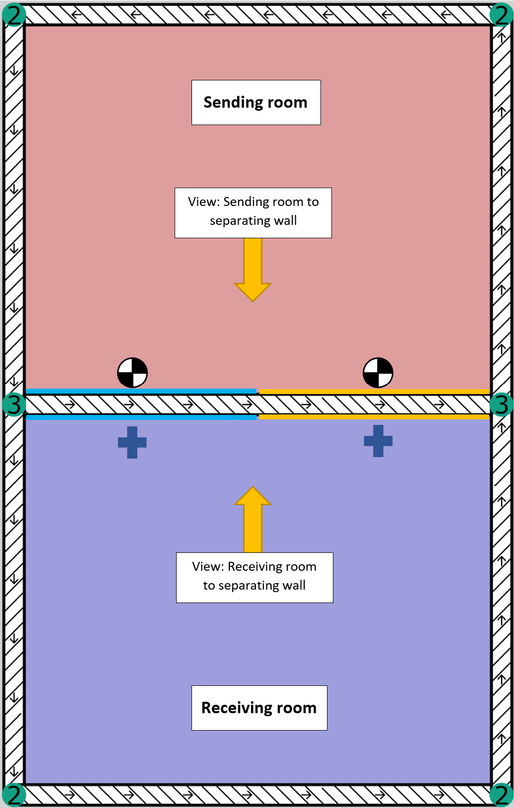
Top view sending room - receiving room with two patches on the separating wall
The following figure "View of the separating wall from the sending room" shows the view of the separating wall from the sending room. A receiver is located in the center of each patch.
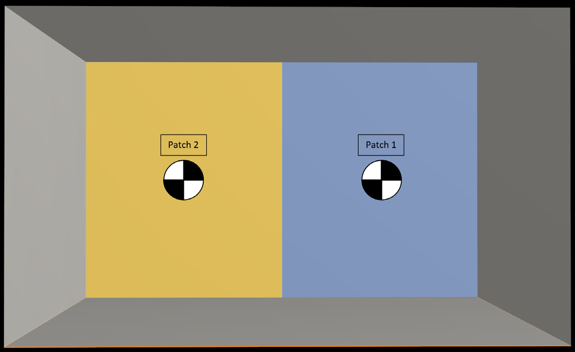
View of the separating wall from the sending room
During the room acoustic calculation (CadnaR) in the sending room, a sound pressure level Lp,SR is determined for the receiver at the patches. From the sound pressure level, a sound power level Lw,RR is determined for the respective point source in the receiving room via the calculation (see Transmission through a separating wall (ISO 12354)) in CadnaB.
The figure below shows the view of the separating wall from the receiving room. In the center of the patches are the point sources assigned to the couplings.
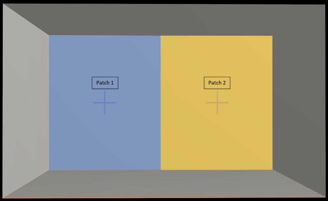
View of the separating wall from the receiving room
A room acoustic calculation for the receiving room is then performed in CadnaR.
Note
For interoperability, only the couplings on the separating component are taken into account.
Coupling grid in practice
In practice, the grid spacing of the coupling grid (see Project) is set in such a way that there are considerably more than two couplings on an ordinary separating wall. A grid spacing of 0.5 m is default. The fine mesh size is directly related to the computational effort and the accuracy of the results provided by the software systems.
The figure below shows a separating wall (width 5 m, height 3 m) with a practical grid division with the width of 1.0 m.
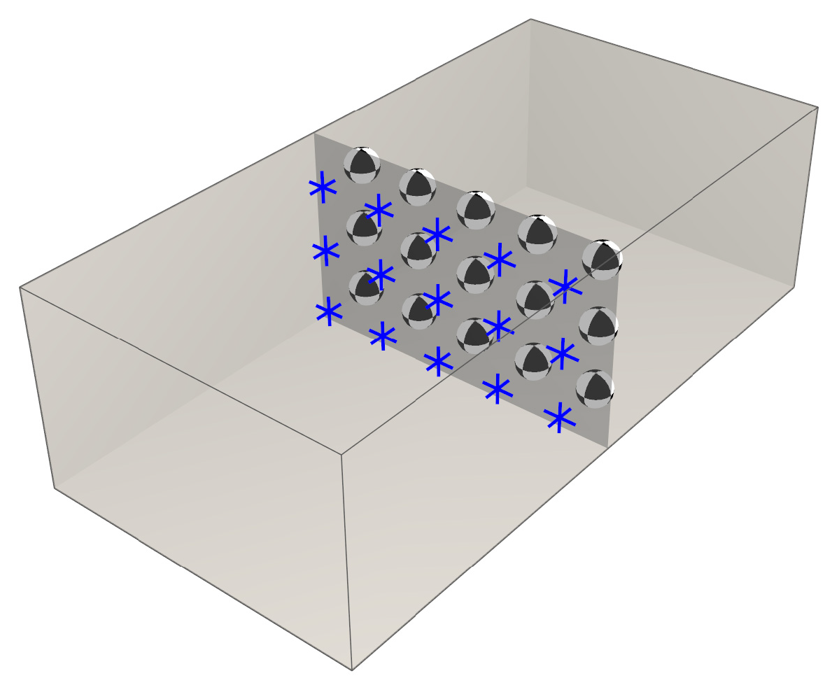
Separating wall with practical grid division
Transmission through a separating wall (ISO 12354)
The airborne sound transmission via separating or flanking components is implemented in CadnaB in connection with interoperability via the following formula. The calculation is done separately for each coupling.
$$
\large L_{W,RR} = L_{p,SR} + C_{Area} - R
$$
\(L_{W,RR}\quad -\) Sound power level in the receiving room
\(L_{p,SR}\quad\ \ -\) Sound pressure level in the sending room
\(C_{Area}\quad\ \ -\) Area correction
\(R\qquad\quad -\) Sound reduction index
Depending on the transmission situation, the sound reduction index R is replaced by \(R'\), \(R_{ges}\) or \(R'_{ges}\).
\(R' \qquad\) apparent sound reduction index of one construction; Consideration of the flanking transmission
$R_{ges} \quad\ $ total sound reduction index; Consideration of all elements in the separating component
$R'_{ges} \quad\ $ total apparent sound reduction index; Consideration of all elements in the separating component and the flanking transmission
Note
The situ correction is considered in this transmission calculation only at the flank components (see section Structural reverberation time, \(R_{situ}\) correction).
Note
The Waterhouse correction is neglected in interoperability.
Determination of the noise level of the façade walls (DIN 4109)
With the calculation standard DIN 4109 set, a sound level is determined for each coupling at the façade walls of the CadnaB Building in CadnaA during the interoperability between CadnaA and CadnaB. The maximum sound level in front of the respective CadnaB walls is selected and assigned as noise level to the walls in CadnaB during synchronization.
Determination of the noise level of the façade walls (ISO 12354)
With the ISO 12354 calculation standard set, a sound level is determined for each coupling on the façade walls of the CadnaB Building in CadnaA in the case of interoperability between CadnaA and CadnaB. From the sound levels, an average sound level is formed for each façade wall, via the energy balance between the inside and outside.
Averaging over the energy balance
Calculation per patch:
-
Determination of the linear sound pressure level or rating level on the outside of the component Lp,i (CadnaA).
-
For calculation of airborne sound transmission from outside to inside, see Explanation of the transmission calculation at a coupling
Note
If values for the sound reduction index are not available for all third octaves between 100 Hz and 5000 Hz in a construction, the band is extended with the last available value at the lower or at the upper end of the third octave band.
-
A-weighting of the sound level on the inside.
-
Calculation of a single-number value by energetic addition Li.
-
Determination of a sound energy: $$ \large E_i = 10^\frac{L_i}{10} $$
-
Calculation of a quotient of the determined sound energy and the number of couplings (n) on the wall: $$ \large E_{n,i} = 10^\frac{E_i}{n} $$
-
Calculate a scalar Si per coupling by forming a quotient of the determined sound energy Ei and the sum of all En,i of the couplings of the wall. $$ \large S_i = \frac{E_i}{\sum_{i=1}^{n}E_{n,i}} $$
-
Scaling of the linear sound pressure levels on the outside: $$ \large L_{p,i,S} = 10 \cdot (S_i \cdot 10^{0.1\cdot L_{p,i}}) $$
Calculation for all couplings:
- From the determined linear sound pressure levels on the outside Lp,i,S, an average level Lp,S is formed for each façade wall, which is defined in CadnaB as the noise level for the respective wall. $$ \large L_{p,S} = 10 \cdot \log \left(\frac{1}{n} \cdot \sum_{i=1}^{n} 10^{0.1\cdot L_{p,i,S}} \right) $$
Note
The single number value displayed in CadnaB is A-weighted.