General Tab
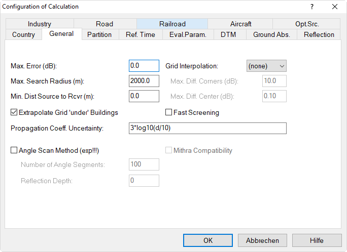
max. Error (dB)
Sound sources, whose contribution to the level at the receiver point is negligible, will be ignored in the calculation if the overall error induced by this simplification is not larger than the defined value. Therefore, the larger the maximum permissible error in the final result, the shorter the time required for the calculation.
Procedure
In order to verify which sources can be ignored for a given maximum error, CadnaA applies the following procedure:
- calculation of the partial levels of all sources based on the geometrical divergence only (e.g. Adiv of ISO 9613-2),
- sorting of the sources according to their partial levels,
- For example, with a maximum error of 1 dB, all sources that contribute less than this amount to the total sum level will be ignored.
This calculation procedure occurs in two steps.
Example
The following examples have a grid of 50*50=2500 point sources with an A-weighted sound power level of PWL=100 dB(A) each. The rays of the sources considered in calculation and the result levels are displayed for maximum errors of 0, 1 and 2 dB.
Example
Path: Examples\Configuration\General\max_error
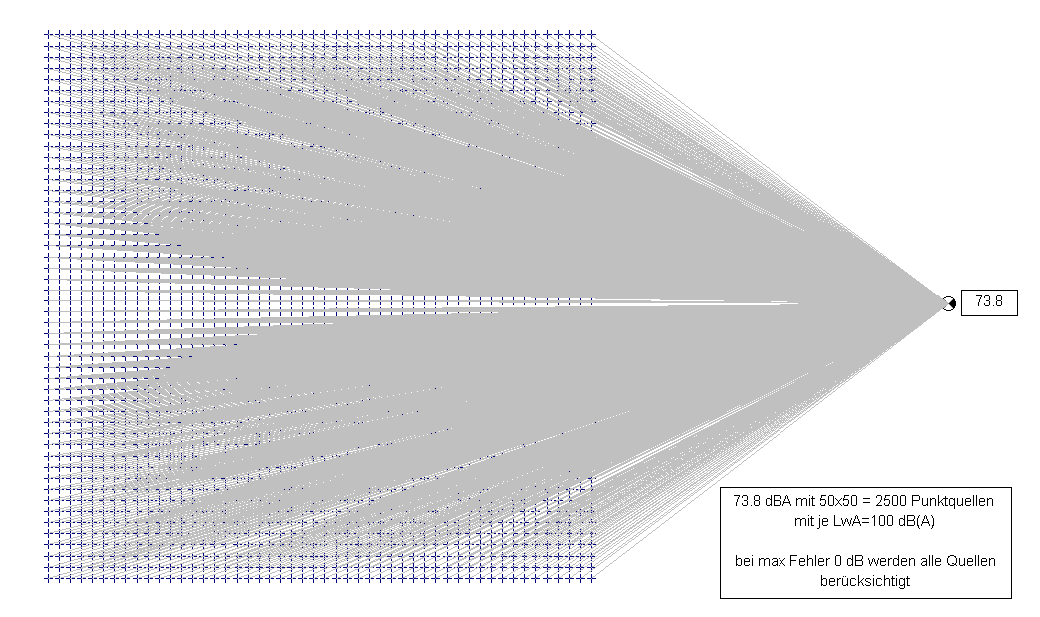 |
max. Error 0 dB resulting level 73.8 dB(A) All sources are taken into account (2500 rays). |
|---|---|
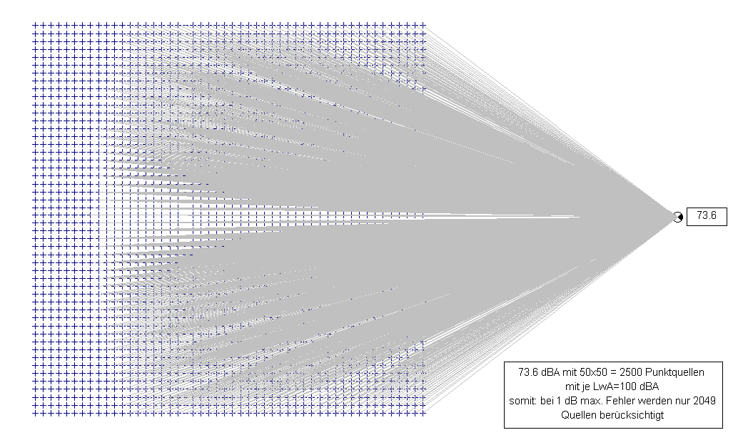 |
max. Error 1 dB resulting level 73.6 dB(A) There are 2049 sources taken into account. |
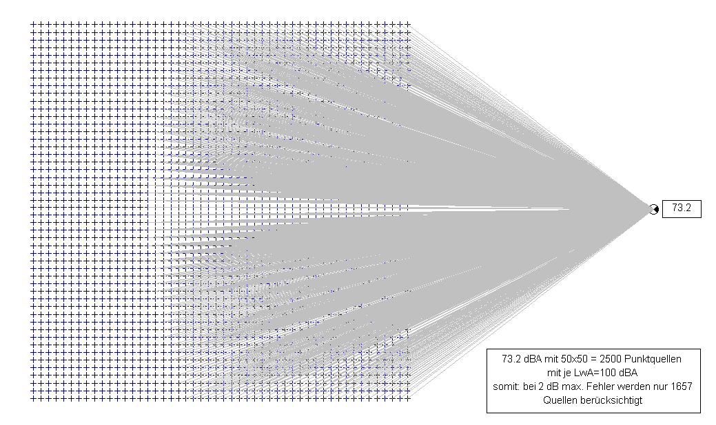 |
max. Error 2 dB resulting level 73.2 dB(A) There are 1657 sources taken into account. |
From the calculation results it can be seen that the level difference compared with the resulting level at a maximum error of 0 dB is usually less than half of the error entered:
| maximum error dB(A) | resulting level dB(A) | difference dB |
|---|---|---|
| 0 | 73.8 | 0 |
| 1 | 73.6 | 0.2 |
| 2 | 73.2 | 0.6 |
| 5 | 71.7 | 2.1 |
This difference is due to just considering of the geometric divergence Adiv when estimating the contribution of each source. Within the final calculation, however, further attenuation terms besides Adiv contribute to the overall attenuation reducing the effect on the resulting level.
Reasonable Values
For expertise work (e.g. noise assessments for legal planning permissions and official approvals) a maximum error of 0 dB shall be used. For noise mapping or other major scenarios, a maximum error of 0 or 1 dB may be useful to reduce the computation time without sacrificing accuracy.
Note
The partial level of sources not considered in the calculation due to the maximum error are not listed on the table Partial Level of a receiver and not in the menu Tables|Partial Level (see Partial Levels and Groups, Partial level at all active receivers).
Note
Furthermore, the sources not considered are also not included in the calculation protocol (see Calculation Protocol).
Restriction with evaluation parameters LmaxD/E/N
If an evaluation parameter of types LmaxD/E/N is selected (see Evaluation Parameters Tab), the maximum error entered when calculating Leq-based levels (e.g. Ld/e/n, Lden...) is ignored and 0.0 dB will be used instead. Therefore, when selecting an evaluation parameter of types LmaxD/E/N make sure that the maximum error entered is 0.0 dB (= standard value) in order to avoid any irritation.
max. Search Radius (m)
By the search radius, a circle is defined around the receiver point. Just the sources inside this circle will be considered in the calculation.
Example
The following examples show that just sources smaller than the search contribute to the receiver level.
Example
Path: Examples\Configuration\General\max_search_radius
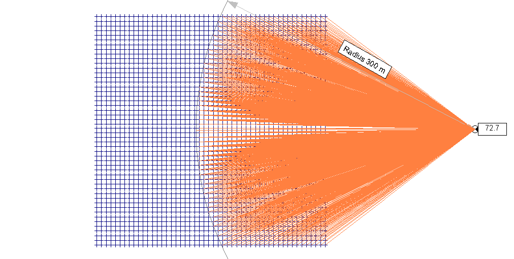 |
search radius 300 m |
|---|---|
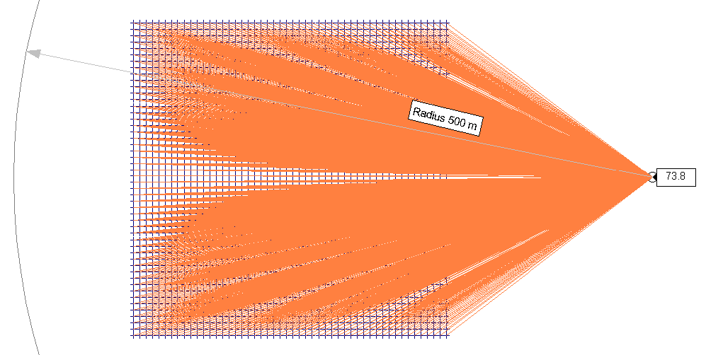 |
search radius 500 m |
Default Value
The default search radius is 2000 m. Depending on the project-specific conditions, a smaller or a larger radius may be useful. A small radius will reduce the calculation time, but may cause that dominant sources outside the search radius may not contribute. By a large search radius more or less all sources are included, but at the expense of a large computation time required without gaining any additional accuracy.
A general value being useful for all kinds of scenarios cannot be given. The table below provides, however, some typical search radii for different scenarios:
| Scenario | Typical Search Radius, value or value range (m) |
| receivers close to source/s(industry, road, railway) | 2000 |
| city center with numerous sources(roads) | 500 |
| rural areas with a few main roads | 5000 |
| large-scale noise mapping projects | 2000 to 5000 |
In any case, the radius shall be increased when loud and presumably dominant sources are located outside of the existing search radius causing level jumps (e.g. with the default search radius of 2000 m). Level jumps caused by single, dominant noise sources can be more easily revealed using the noise grid than being caused by numerous, spatially distributed sources.
Min. Distance Source to Receiver
The minimum distance source-receiver enables to suppress the calculation of propagation near the source. Within this vicinity of the source the same total attenuation as calculated at the minimum distance specified is used causing no increase in overall attenuation with distance in this area.
Example
The following example shows the grid appearance for the minimum distances of 0 and 20 m along a road.
Example
Path: Examples\Configuration\General\min_distance_source_rcvr
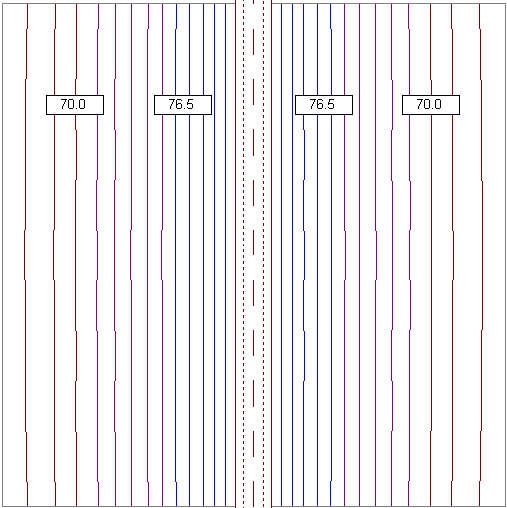 |
minimum distance source to receiver 0 m (default setting) noise contours reach to the emission lines of the source (here: road) |
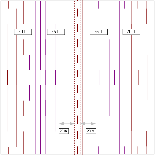 |
minimum distance source to receiver 20 m noise contours start from minimum distance (here in steps of 1 dB) |
Uncertainty
In CadnaA you also have the possibility to evaluate the accuracy of noise prediction. This accuracy depends on the accuracy of the emission values used and the accuracy resulting from the calculation of propagation.
Propagation Coefficient Uncertainty
In addition to the uncertainty of the emission data the uncertainty of the propagation can be taken into account (as e.g. caused by varying meteorological conditions). Enter an expression into the input box „Propagation Coefficient Uncertainty“.
Examples for expressions:
| Expression | Remarks |
| 3 dB | global correction, i.e. no increase with distance d |
| 3*log10(d/10) (Default) |
uncertainty depending on distance, uncertainty is 3 dB at 10 m distance, reference distance d0=10 m |
| max(1, 2*log10(d/1)-3) | based on a legal act when predicting the noise impact from wind turbines in the German state of Brandenburg, reference distance d0=1 m |
Available Abbreviations
In addition to the operators (see Chapter 5 - Operators & Functions in CadnaA manual „Attributes, Variables, and Keywords“) the following additional attributes are available:
- d: 3D-distance source-receiver
- d2: 2D-distance source-receiver
plus all further operators for expressions available in CadnaA.
Note
By default, the calculated sound levels are not altered just by specifying a standard deviation Sigma or a propagation coefficient uncertainty. This requires to select or enter a suitable parameter or expression on tab „Evaluation Parameter“ (see Evaluation Parameters Tab).
Standard Deviation Sigma
The source-specific uncertainty is specified by entering a standard deviation Sigma (dB) on the dialog Memo Window of each individual source. In case the sound power level of the source has been measured, the standard deviation for grades 1, 2 or 3 can be used (according to ISO 3740 series).
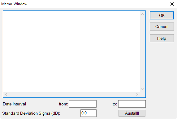
Dialog Memo-Window (accessible via each source dialog)
Make sure that at least one of the evaluation parameters SigmaD/SigmaE/SigmaN (for Day|Evening|Night) on the tab „Evaluation Parameter“ has been selected. The calculation of the Sigma values for single receiver (see Receiver Grid) occurs using the command Calculation|Calc or by clicking on the calculator symbol on the toolbar. The results are displayed on the dialog Receiver or on the Result Table (see Result Table). The distribution of the uncertainty can be displayed as well on the grid resulting from a grid calculation (menu Grid|Calc Grid, see Receiver Grid).
Example
Path: Samples\Infos\Uncertainty.pdf
In Pro-2002 it is shown how to evaluate the uncertainty of levels based on the uncertainty of sources and the uncertainty of propagation. The procedure using the data structure as implemented in CadnaA is demonstrated by an example.
Extrapolate Grid ’under’ Buildings
This option enables a seamless transition of the grid - regardless of the type of appearance selected (see Grid Appearance) - to the borders of closed polygons (such as of object types „Building“, „Area Source“, and „Parking Lot“). This is accomplished by interpolating the grid level values up to the first grid point inside polygon area. When calculating the levels at these grid points, the screening effect by the actual obstacle is not considered (i.e. an extrapolation of the free-field level occurs). This option is enabled by default.
Examples
Example
Path: Examples\Configuration\General\extrapolate_grid
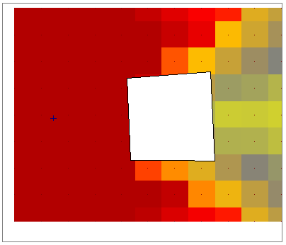 option activated: extrapolation occurs up to the 1st grid point laying inside the building |
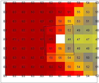 option activated: as before, with transparent building and with grid values |
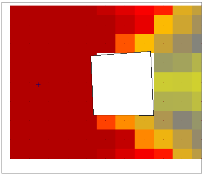 option deactivated: white gaps outside the building are due to the next grid point laying inside the building |
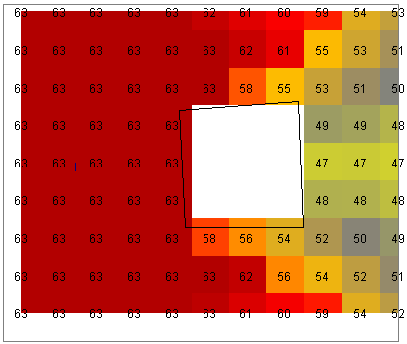 option deactivated: as before, with transparent building and with grid values |
It is recommended to deactivated the option „Extrapolate Grid ’under’ Buildings“ with the grid appearance option „Lines of Equal Sound Level“ selected in conjunction with the activated option „Exclude Buildings“ on menu Grid|Specifications|Options (see Grid Specification).
Calculation of Terrain Height
With the option „Extrapolate Grid ’under’ Building“ activated this also applies to the calculated terrain height level at each grid point
Vertical Grid
This option has no effect at vertical grids, i.e. there is no extrapolation of the grid calculated in the vertical plane grid in front of the facade the building’s interior area. Therefore, lower levels may be displayed - in particular with grid appearance options „Lines of Equal Sound Level“ and „Areas of Equal Sound Level“ - on the vertical grid in front of a facade grid due to the missing extrapolation to the building’s interior.
Grid Interpolation
If this option with the setting n*n is selected, the level calculation occurs starting at each of the (n+1) grid points of the horizontal grid as specified on menu Grid|Specification and at the center point of each rectangle delimited by those four points.
The grid interpolation is not applied to vertical grids.
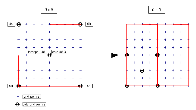
Option "Grid Interpolation": approach when the transitionfrom a rectangle of size 9*9 to size 5*5 occurs
If either of the following conditions are not met for each rectangle delimited by the four calculated points, this rectangle is subdivided into four equal squares and the check is repeated for each of these new four rectangles. If any of these conditions is still not met, a further subdivision occurs recursively until, in the end, the conditions are met or all grid points have been taken into account in the calculation based on the grid specification.
Conditions
The conditions are:
- The difference between the largest and the smallest level calculated at the four corners of the rectangle is, at most, equal with the specified maximum value (default value: 10 dB).
Note
The default value of 10 dB ensures that - in case of significant extra attenuation between the corners (e.g. by large obstacles) - a further subdivision occurs.
- The mean level calculated from the levels at the two corner points of each diagonal shall not differ from the level at the center point by more than the specified maximum deviation (default value: 0.1 dB). This condition must be fulfilled for both diagonals.
Note
The default value of 0.1 dB is - in general - exceeded if additional attenuations on the diagonals between the corners and the center are caused, e.g. by a screening obstacle.
When these conditions are fulfilled, the interpolated values inside the rectangle match sufficiently with the real values and the levels at the remaining grid points inside the rectangle are interpolated from the levels calculated at the four corner points.
Fast Screening
When selecting this option, an approximative method for the screening calculation when using RLS90 or Schall03 (1990) is applied causing an acceleration of the screening calculation. In this case, however, the calculation applied is longer compliant with those guidelines.
Note
Do not use this option with other calculation standards or source types (in particular not with point, line and area sources) as this may cause irregular results.
By this procedure, no detailed calculation by scanning each for each obstacle in the ray’s path occurs, but a given parabolic ray path is used. Only those buildings exceeding this path will contribute to the screening effect while the others are not even checked for.
In the vertical cross-section (see Cross Section) only those obstacles are shown contributing to the screening effect. Those not being intersected by the ray path are not displayed.

"fast screening" activated: On the sectional view of a rayonly a limited number of obstacles are displayed(detailed section near the source).

"fast screening" deactivated: On the sectional view of a rayall obstacles are displayed as all are included in the screening calculation(detailed section near the source)
Calculation Strategies
The following method is used in CadnaA by default.
The ray paths between sources and receivers are constructed in a deterministic way. Extended sources are subdivided dynamically applying the projection method. The source segments represented by a single ray are shorter at small receiver distances and large at large receiver distances. Screening objects and all gaps between them produce at least one single ray (see also chapter Projection at extended Sound Sources). With the option „Angle Scan Method“ deactivated (see below) this method is used.
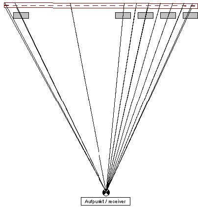
Method with projection to subdivide extended sources dynamically
Angle Scanning (AS)
Alternatively, with the option „Angle Scan Method“ activated, the procedure described in the following will be used. In this case, the calculation of the receiving levels is carried out using rays emitted at constant angular steps, starting from the receiver point to the source. Only those objects intersected by the ray’s path contribute to the screening effect. Point sources situated within the angle cone are virtually transferred to the ray’s path.
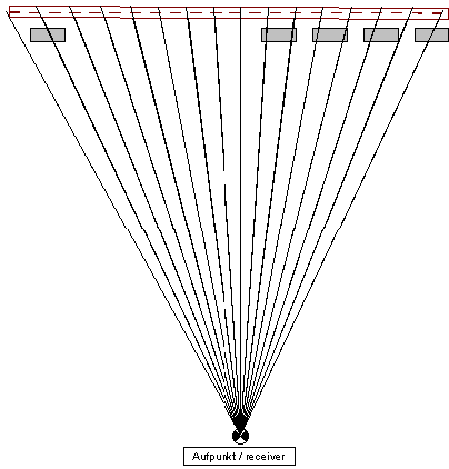
Angle Scanning Method: Rays start from the receiver and are spaced at equal angular steps
Options
- Number of Angle Segments: default value 100, resulting in 360°/100=3.6° steps between rays
- Reflection depth: With a reflection depth of zero, obstacles behind the first reflector in direction of the ray are not seen, irrespective of the reflection order specified and when the first reflector detected was not reflective, based on its dimensions. Thus, the specification of the reflection depth represents the number of potential reflectors which can be ignored in ray direction because of their dimensions. However, at least a single additional reflector is taken into account in any case.Example: In order to detect reflector no. 4, a reflection depth of at least 3 must be specified.
Note
With the option „Angle Scan Method“ activated the settings on the „Partition“ tab are no longer relevant (see Partition Tab).
Note
With the option „Angle Scan Method“ activated, the function „Pass-by of individual Vehicles“ is not available, see Pass-By of individual Vehicles.
Mithra Compatibility
When the option „Mithra Compatibility“ is activated, all the approximations used in the software Mithra are also used in CadnaA-Mithra. This is the mode that should be used to load MITHRA projects using CadnaA-Mithra and to obtain the same results as with MITHRA.
Note
The check box is only available if the option CadnaA-Mithra has been purchased.
Within the MITHRA compatible calculation - among others - additional screening will be taken into account, see the barriers with special crowning in CadnaA-Mithra (see Barrier with special crowning).