Particle Model

With the particle model, a large number of so-called "sound particles" is emitted randomly by the source into all directions. In this case, the location of the receivers or of the grid point is not relevant, but just the direction into which the respective sound particle is radiated. Every sound particle represents a solid angle of a spherical wave with the corresponding sound energy of the sound source. The sound particles are pursued up to the specified maximum runtime or order of reflection. Obstacles in particle direction can be absorbing, scattering and transmitting while the room surfaces may have an absorbing and possibly a scattering effect only. The receiver level in a volume element (voxel) is obtained by summation of all energy contributions.

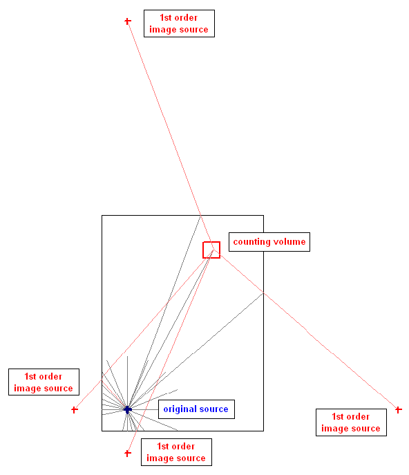
Calculation Principle of the Particle Model: Particle Paths and Counting Volume

The calculation can be split into four parts:

1. In a first step, the rays emitted by the sources are generated randomly. The algorithm applied ensures that the directional distribution of these rays is random, also with a large number of rays and many iterations. There are as many particles - distributed over all sources - produced as specified in the configuration, section „Particles“ (default 100,000 particles, absolute). The location of point sources resulting from the segmentation of line and area sources is also at random. Both procedures ensure that no systematic spatial level differences occurs (neither negative, nor positive differences). At a low particle numbers, however, level differences may occur between different calculation runs with the same source arrangement (described by the standard deviation).

2. In a second step, the path of the generated particles produced is pursued within the room space up to the specified maximum runtime or order. The direction of the particles reflected at room surfaces or at obstacles is determined according to the laws of geometrical acoustics. The energy which every particle represents is decreased by the absorptive properties of the reflector. If scattering at the room‘s surfaces or at obstacles can occur (see „Particle Model“ tab), the incident particles are scattered or reflected as specified by the scattering coefficient. Here, a spatial distribution of the scattered energy according to Lambert's cosine law is used ("ideal diffuse"). If transmission of obstacles can occur (see „Particle Model“ tab), the incident particles are transmitted or reflected as specified by the transmission coefficient. There is no change of direction for transmitted particles.

3. In the third step, the energy of all particles inciding into a distinct counting volume is summed up. The individual counting volume represents a 3D volume cell defined by the dimensions of the volumetric grid. Per default, the counting volume is 0.125 m³ (with dimensions 0.5*0.5*0.5 m). The penetrated length within a voxel is used to compensate for the diverging solid angles for different directions of incidence of a particle.

4. In the fourth step it is checked at the end of the current iteration whether the maximum standard deviations (in dB) specified in the configuration for voxels and/or for receivers (see Configuration, "Calculation" tab) is met (break condition). If not, a further iteration is executed. After each iteration, this test is performed again until the criteria for the standard deviation are fulfilled.

Note

With particle model no rays from the source to the receivers can be displayed (see Receiver, option „Generate Rays (as Auxiliary Polygons)") since there are no distinct rays emitted to those receivers. For the same reason, in this case the „emission sound pressure level LpA (dB) at a workplace“ for sources which have been assigned to a receiver point cannot be considered in the receiver level (see also „Particle ping-pong“, chapter 3D-View).

Combined Procedure „Image Sources --> Particles“

With the combined procedure „Image Sources --> Particles“ the image source procedure is applied up and including the order n specified in section „Image Sources“. For higher orders (starting from n+1) up to the specified maximum runtime or order of reflection the particle model is used (see Configuration).

Applying the combined procedure enables to accelerate the calculation of complex scenarios with large numbers of screening obstacles, without neglecting the energy contributions due to higher orders of reflections entirely.

Note

When using the combined procedure „Image Sources --> Particles“, however, the emission sound pressure level LpA (dB) at a workplace of sources assigned to a receiver point is considered in the receiver level. In this case the direct sound of the referred source is determined from the emission sound pressure level, while the direct sound of further sources and the reflected sound results from ray tracing.

Application Notes

The calculation results for the procedures „Image Sources“ (without diffraction, see Image Source Model) and „Particles“ hardly differ from each other, provided a sufficient number of particles is used.

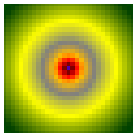	Image Sources max. order 0 grid spacing 1*1 m Example: Files/Tutorial/Chap 7_2/Table 1/ImageSources - ReflectOrd 0.cni
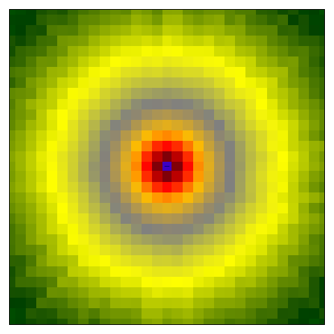	Particle Model max. order 0 voxel distance 1*1*1 m number of particles: 1 million (default setting) Example: Files/Tutorial/Chap 7_2/Table 1/Particle Model 1 Mio - ReflectOrd 0.cni
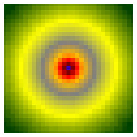	Particle Model max. order 0 voxel distance 1*1*1 m number of particles: 10 million Example: Files/Tutorial/Chap 7_2/Table 1/Particle Model 10 Mio - ReflectOrd 0.cni

Table 1: Comparing procedures „Image Sources“ vs. „Particles“

With the particle model it is no useful to reduce the voxel distance to achieve better results. Instead, an increased number of particles is required to ensure a better quality of the results.

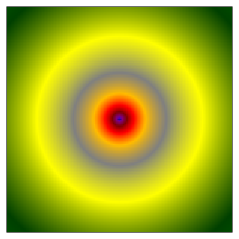	ImageSources max. order 0 grid spacing 0.2*0.2 m Example: Files/Tutorial/Chap 7_2/Table 2/ImageSources - ReflectOrd 0 - grid 0.2x0.2 m.cni
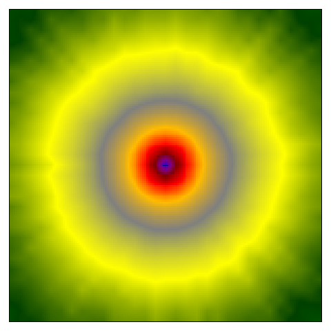	Particle Model max. order 0 voxel distance 1*1*1 m number of particles: 1 million Example: Files/Tutorial/Chap 7_2/Table 2/Particle Model 1 Mio - ReflectOrd 0 - Voxel 1x1x1 m.cni
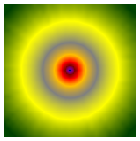	Particle Model max. order 0 voxel distance 1*1*1 m number of rays: 10 million Example: Files/Tutorial/Chap 7_2/Table 2/Particle Model 10 Mio - ReflectOrd 0 - Voxel 1x1x1 m.cni

Table 2: Comparing Image Sources/Particles using a smaller grid or voxel spacing

With the number of particles being too small, the local level is with increasing distance from the source determined by a few particles only, resulting in a notably high statistical uncertainty. Moreover, at a small number of particles, due to the particles emitted into random directions, diverging level distributions result for the grid upon repetitive calculation runs.

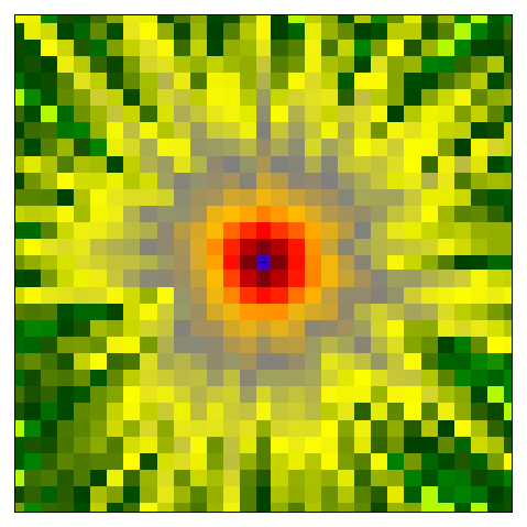	Particle Model max. order 0 voxel distance 1*1*1 m number of particles: 10.000 Example: Files/Tutorial/Chap 7_2/Table 3/Particle Model 10000 - ReflectOrd 0 - Voxel 1x1x1 m.cni
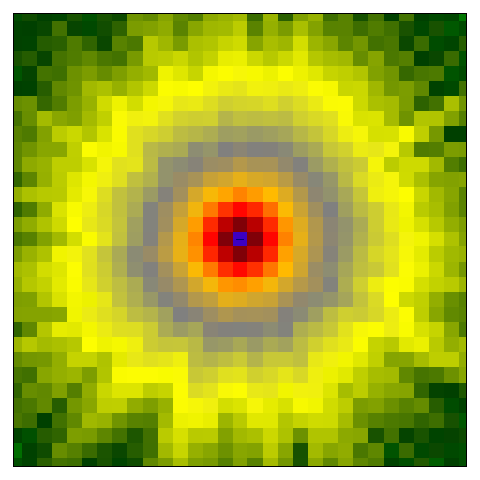	Particle Model max. order 0 voxel distance 1*1*1 m number of particles: 100.000 Example: Files/Tutorial/Chap 7_2/Table 3/Particle Model 100000 - ReflectOrd 0 - Voxel 1x1x1 m.cni

Table 3: Particle model at low numbers of particles

Note

The same situation with the number of particles being 1.000.000 and 10.000.000 have been discussed in table 1 already, see there.