Calculate Virtual Acoustic Camera

The virtual acoustic camera can be used to show the direction from which sound reaches a receiver. This can be used to localize sound sources and their reflections, investigate sound distributions and carry out acoustic optimizations in various application areas.

Calculation of the virtual acoustic camera

There are two ways to calculate the virtual acoustic camera:

• Including the calculation when using other calculation functions (see "General" tab Virtual Acoustic Camera). The virtual acoustic camera is available in addition to the other calculation results. Higher disk storage requirements, larger CadnaR file.
• Explicit calculation using the calculation function in the menu Calculation|Calculate virtual acoustic camera. Only the virtual acoustic camera is calculated. Grids, voxel grids etc. are then not available as calculation results. Less disk storage required, smaller CadnaR file.

Display of the virtual acoustic camera

There are two ways to display the virtual acoustic camera:

• from the object dialog of the receiver with the corresponding button, see Receiver Button „Virtual Acoustic Camera“
• with the 3D view open and the receiver selected via CTRL+F9 (or via the Camera menu), see 3D-View Camera menu

Display modes and settings

Dynamic and absolute display mode,ALT+mouse wheel

There are two display modes for the virtual acoustic camera:

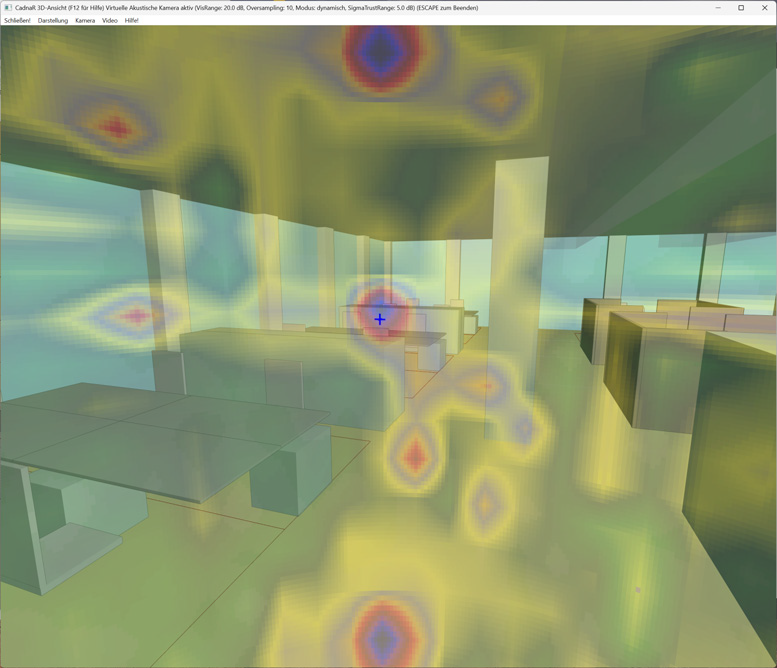
• Dynamic (default): the color palette is dynamically adapted to the visible range. Mouse wheel for quick adjustment of the visible range. This mode is used to identify hotspots or main directions of sound incidence.
• absolute: the exact color assignment defined in the color palette is used. This mode is ideal for comparing various planning scenarios.

Switching between the two modes via the Camera menu or with ALT+mouse wheel.

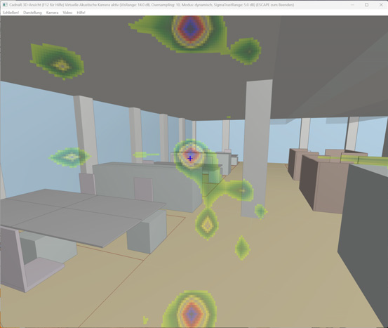Mode: dynamic, planning scenario 1	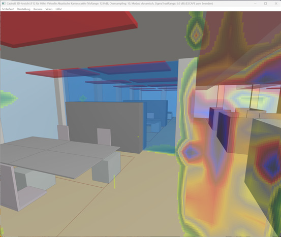Mode: dynamic, planning scenario 2
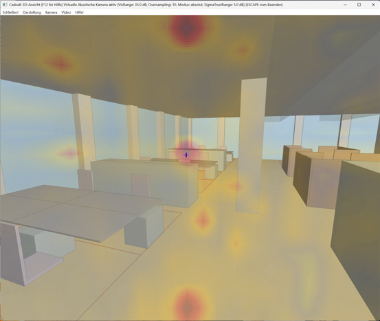Mode: absolute, planning scenario 1	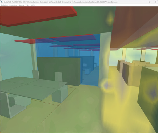Mode: absolute, planning scenario 2

Visible range, VisRange,Mouse wheel

In both display modes, the visible range can be adjusted using the mouse wheel, the corresponding VisRange parameter is displayed in the title bar of the 3D view.

• Visible range in dynamic mode: The loudest incidence direction corresponds to the 'loudest' color in the palette, while subtracting the 'VisRange numerical value' from it corresponds to the 'quietest' color.
• Visible range in absolute mode: the visible range starts at the level of the loudest incidence direction and extends downward by the 'VisRange numerical value'.

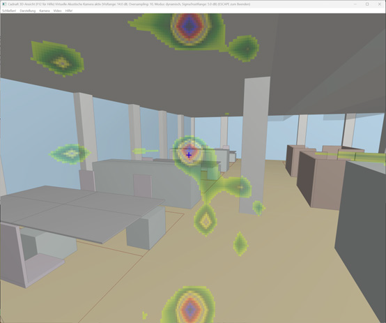Mode: dynamic,Visible range VisRange: 14 dB	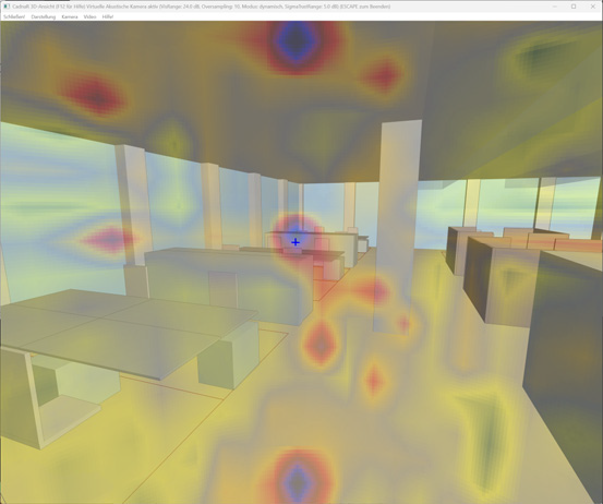Mode: dynamic, Visible range VisRange: 24 dB
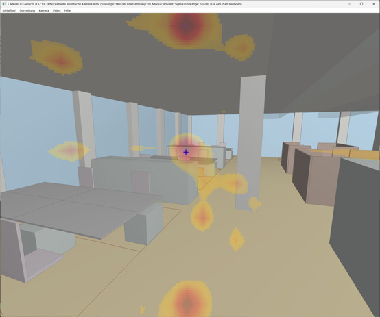Mode: absolute, Visible range VisRange: 14 dB	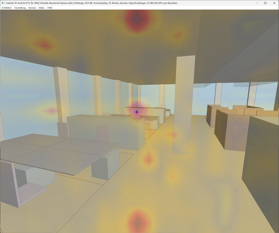Mode: absolute, Visible range VisRange: 24 dB

Oversampling CTRL+mouse wheel

Oversampling can be set in both display modes via the Camera menu or using CTRL+mouse wheel. Oversampling =1 is used by default, which corresponds to no oversampling or the display of raw data. High oversampling undoubtedly produces more visually appealing graphics. However, it is always advisable to take a look at the raw data, especially in the event of any implausibilities.

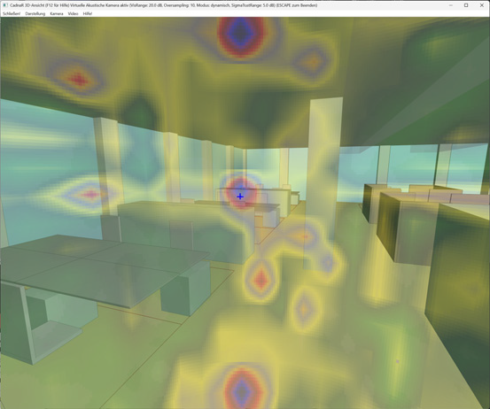Oversampling: 10

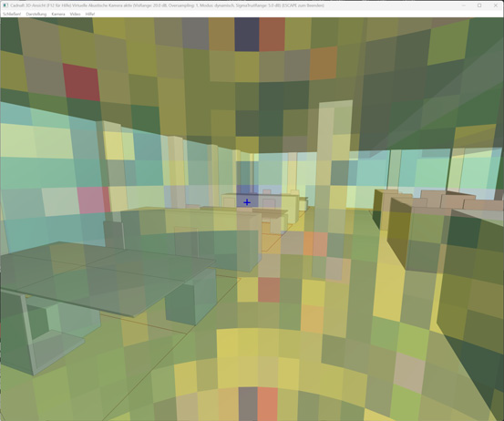Oversampling: 1, raw data

Color palette and progressive colors

An individual color palette for the virtual acoustic camera can be set in the Grid|Appearance menu (see Grid Appearance). By default, the color palette of the level grid is also used for the virtual acoustic camera. For the handling of progressive colors, the logic applied to the level grids is also applied for the virtual acoustic camera (see Grid Appearance Progressive Colors).

Incidence direction-dependent result uncertainty, SigmaTrustRange,SHIFT mouse wheel

When using the particle model, the repeatability of the A-level at the receiver is ensured by using the standard deviation for receivers (see Configuration). However, the virtual acoustic camera evaluates the particles depending on the direction of incidence. As a result, individual directions of incidence can have a higher uncertainty of results, which is expressed in an increased standard deviation for these directions of incidence. By default, directions of incidence with a standard deviation above 5 dB(A) (SigmaTrustRange = 5 dB in the title bar of the 3D view) are not displayed. For standard deviations up to 0.1 * SigmaTrustRange (0.5 dB(A) by default), the color is attenuated by increasing its transparency. More accurate results appear without transparency adjustment. The SigmaTrustRange parameter can be changed in the 3D view with SHIFT + mouse wheel.

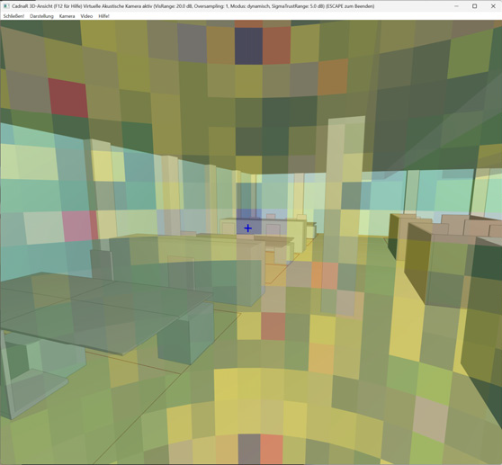SigmaTrustRange: 5dB,long calculation time, many particles	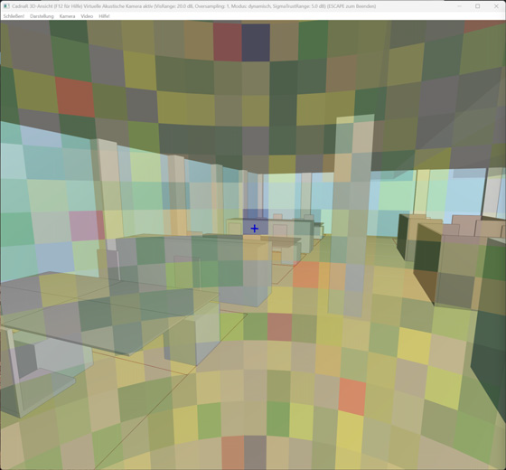SigmaTrustRange: 5dB,short calculation time, few particles
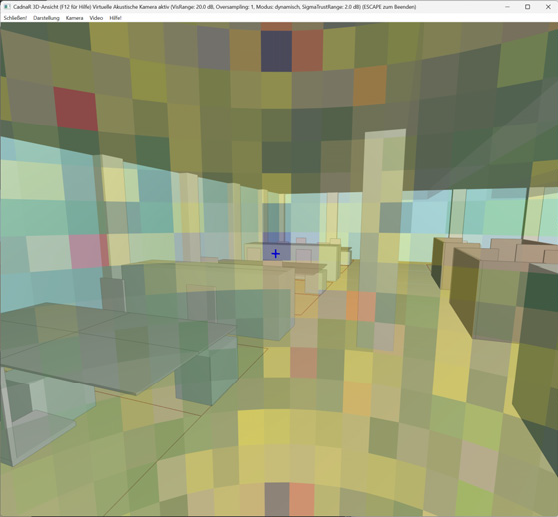SigmaTrustRange: 2dB,long calculation time, many particles	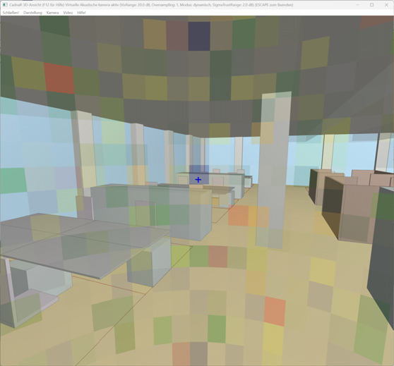SigmaTrustRange: 2dB,short calculation time, few particles

The previous raw data example clearly shows::

• With a (sufficiently) high number of particles, the differences in transparency with SigmaTrustRange 5dB and 2dB are minimal or unnoticeable.
• With a low number of particles, SigmaTrustRange can help to suppress uncertain immission directions.

Presets

The camera presets can be used to save and load the virtual acoustic camera including all settings (receiver, mode, visible range, etc.) and can also be used in the Plot Designer, for example.

Additional technical information

Immission directivity

The immission directivity is defined in the same way as the emission directivity (see Directivities (local), see Point Source) via the angle of rotation phi and theta. The increments in phi and theta can be set in the calculation configuration (see "General" tab). A higher resolution requires more disk storage space, a higher number of particles and longer calculation times.

particle model, voxel and receiver

When calculating with the particle model, the immission directivity is identical for all receivers located within the same voxel. The virtual acoustic camera always shows the perspective from the center of the voxel.

image sources, hybrid methods

When using the image source model or hybrid methods (image sources -> particles), the virtual acoustic camera is displayed from the exact receiver location (not from the voxel center).

Additional handling information

An open object dialog prevents the switching of variants. If the virtual acoustic camera was opened via the button in the object dialog of the receiver, the object dialog must be closed again before the variants can be switched.